검색결과 리스트
CORDIC에 해당되는 글 1건
- 2010.03.24 Cordic 알고리즘
Origianl From : Wikipedia CORDIC
CORDIC은 "for COordinate Rotation DIgital Computer"의 약자로 1959년 Jack E. Volder에 의해 처음 개발 되었고 HP의 John Stephen Walther가 일반화 하였다.
CORDIC은 hyperbolic, trigonometric function, Exponential, Logarithms, Multiplication, Division, Square Root 등 다양한 연산을 Bit-Shift, Addition의 단순한 구조로 구현 가능하도록 하는(멀티플라이어가 필요 없는) 하드웨어에 최적화 된 알고리즘 이다.
(단 반복적인 Iteration이 요구되어 Polynomial 연산법 등에 비해 속도는 저하 될 수 있다.)
원래 CORDIC은 이진수 체계를 가지는 시스템에서 적용하기 위해 개발되었으나 1970년대에는 10진(decimal) CORDIC이 포켓 계산기에서 광범위하게 사용되기 시작하였다.(대부분 BCD코드 사용)
동작방식
CORDIC can be used to calculate a number of different functions. This explanation shows how to use CORDIC in rotation mode to calculate sine and cosine of an angle, and assumes the desired angle is given in radians and represented in a fixed point format. To determine the sine or cosine for an angle β, the y or x coordinate of a point on the unit circle corresponding to the desired angle must be found. Using CORDIC, we would start with the vector v0:

In the first iteration, this vector would be rotated 45° counterclockwise to get the vector v1. Successive iterations will rotate the vector in one or the other direction by size decreasing steps, until the desired angle has been achieved. Step i size is Artg(1/(2(i-1))) where i 1,2,3,….

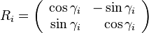
More formally, every iteration calculates a rotation, which is performed by multiplying the vector vi − 1 with the rotation matrix Ri:

The rotation matrix R is given by:
Using the following two trigonometric identities
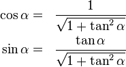
the rotation matrix becomes:
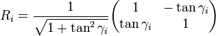
The expression for the rotated vector vi = Rivi − 1 then becomes:
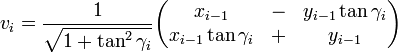
where xi − 1 and yi − 1 are the components of vi − 1. Restricting the angles γi so that tanγi takes on the values  the multiplication with the tangent can be replaced by a division by a power of two, which is efficiently done in digital computer hardware using a bit shift. The expression then becomes:

where
and σi can have the values of −1 or 1 and is used to determine the direction of the rotation: if the angle βi is positive then σi is 1, otherwise it is −1.
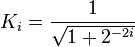
We can ignore Ki in the iterative process and then apply it afterward by a scaling factor:
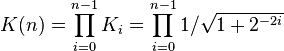
which is calculated in advance and stored in a table, or as a single constant if the number of iterations is fixed. This correction could also be made in advance, by scaling v0 and hence saving a multiplication. Additionally it can be noted that
to allow further reduction of the algorithm's complexity. After a sufficient number of iterations, the vector's angle will be close to the wanted angle β. For most ordinary purposes, 40 iterations (n = 40) is sufficient to obtain the correct result to the 10th decimal place.
The only task left is to determine if the rotation should be clockwise or counterclockwise at every iteration (choosing the value of σ). This is done by keeping track of how much we rotated at every iteration and subtracting that from the wanted angle, and then checking if βn + 1 is positive and we need to rotate clockwise or if it is negative we must rotate counterclockwise in order to get closer to the wanted angle β.

The values of γn must also be precomputed and stored. But for small angles, arctan(γn) = γn in fixed point representation, reducing table size.
As can be seen in the illustration above, the sine of the angle β is the y coordinate of the final vector vn, while the x coordinate is the cosine value.
소프트웨어 구현 :
The following is a MATLAB/GNU Octave implementation of CORDIC that does not rely on any transcendental functions except in the precomputation of tables. If the number of iterations n is predetermined, then the second table can be replaced by a single constant. The two-by-two matrix multiplication represents a pair of simple shifts and adds. With MATLAB's standard double-precision arithmetic and "format long" printout, the results increase in accuracy for n up to about 48.
function v = cordic(beta,n)
% This function computes v = [cos(beta), sin(beta)] (beta in radians)
% using n iterations. Increasing n will increase the precision.

if beta < -pi/2 || beta > pi/2
    if beta < 0
        v = cordic(beta + pi, n);
    else
        v = cordic(beta - pi, n);
    end
    v = -v; % flip the sign for second or third quadrant
    return
end

% Initialization of tables of constants used by CORDIC
% need a table of arctangents of negative powers of two, in radians:
% angles = atan(2.^-(0:27));
angles =  [  ...
    0.78539816339745   0.46364760900081   0.24497866312686   0.12435499454676 ...
    0.06241880999596   0.03123983343027   0.01562372862048   0.00781234106010 ...
    0.00390623013197   0.00195312251648   0.00097656218956   0.00048828121119 ...
    0.00024414062015   0.00012207031189   0.00006103515617   0.00003051757812 ...
    0.00001525878906   0.00000762939453   0.00000381469727   0.00000190734863 ...
    0.00000095367432   0.00000047683716   0.00000023841858   0.00000011920929 ...
    0.00000005960464   0.00000002980232   0.00000001490116   0.00000000745058 ];
% and a table of products of reciprocal lengths of vectors [1, 2^-j]:
Kvalues = [ ...
    0.70710678118655   0.63245553203368   0.61357199107790   0.60883391251775 ...
    0.60764825625617   0.60735177014130   0.60727764409353   0.60725911229889 ...
    0.60725447933256   0.60725332108988   0.60725303152913   0.60725295913894 ...
    0.60725294104140   0.60725293651701   0.60725293538591   0.60725293510314 ...
    0.60725293503245   0.60725293501477   0.60725293501035   0.60725293500925 ...
    0.60725293500897   0.60725293500890   0.60725293500889   0.60725293500888 ];
Kn = Kvalues(min(n, length(Kvalues)));

% Initialize loop variables:
v = [1;0]; % start with 2-vector cosine and sine of zero
poweroftwo = 1;
angle = angles(1);

% Iterations
for j = 0:n-1;
    if beta < 0
        sigma = -1;
    else
        sigma = 1;
    end
    factor = sigma * poweroftwo;
    R = [1, -factor; factor, 1];
    v = R * v; % 2-by-2 matrix multiply
    beta = beta - sigma * angle; % update the remaining angle
    poweroftwo = poweroftwo / 2;
    % update the angle from table, or eventually by just dividing by two
    if j+2 > length(angles)
        angle = angle / 2;
    else
        angle = angles(j+2);
    end
end

% Adjust length of output vector to be [cos(beta), sin(beta)]:
v = v * Kn;
return


RECENT COMMENT