Lambertian surface,램버시안 표면


물체 표면의 각에 따른 반사광의 세기가 법선과 반사광의 방향 사이의 각이 코사인 함수값으로 변하는, 단위 입체각에서 모든 방향으로 균일한 광속을 갖는 반사체로 반사 광도가 보는 각도에 관계없이 일정한 표면을 의미한다.

즉, 왼쪽 그림과 같이 모든 방향으로 일정하게 반사되는 표면을 완전확산면, 램버시안 표면이라고 한다.

예를 들면 보름달이나 하얀 종이 같은 것이 완전 확산면에 가깝다.

완전 확산명은 보통 lambertian distribution라고도 불리며 lambertian distribution은 모든 방향에서의 반사되는 빛의 합을 말한다.

by 쿠리다쿠리 2014. 12. 2. 20:40
Manifold (From Wiki...)

수학에서 다양체(多樣體) 혹은 매니폴드(manifold)는 기하학적인 유추를 통해 4차원 이상의 공간을 연구하기 위해 도입된 개념. 국소 유클리드적 위상공간(位相空間)을 일반적으로 위상다양체라 하며, 미분가능 구조를 가진 것을 미분가능다양체 또는 간단히 가미분다양체라고 한다.

어떤 점 근처에서도 유클리드 공간과 닮은 도형을 말한다. 임의의 점 근처에서(국소적으로 locally)는 유클리드 공간과 비슷하지만, 다양체 전체는(전역적으로 globally) 유클리드 공간과 다른 연결 구조를 가지고 있을 수 있다.

이를테면 공간의 곡면이나 평면은 2차원 다양체이다. 또 곡선은 1차원 다양체이다.  

예를 들어, 구면은 충분히 가까이에서 보면 평면, 즉 2차원 유클리드 공간처럼 보인다. 이것은 구면 위에서 사는 작은 개미를 상상하거나, 중세 이전(고대 그리스를 제외하고)에 지구가 평평하다고 생각했던 것을 생각하면 이해하기 쉬울 것이다. 그러나 구면 전체는 특별하게 연결되어 있어, 평면 만으로는 구면을 이해할 수 없다. 평면에 펼쳐 그린 세계지도를 보면 지구를 한 바퀴 돌아서 제자리에 돌아온다는 것을 나타낼 수 없다.

직관적으로 전혀 떠올리기 힘든 집합도 다양체로 취급하여, 기하학적으로 다루는 경우가 있다. 물론, 다양체가 아닌 도형(예를 들면, 페아노곡선, 프랙탈)도 있다.

원은 모든 점에 대해서 국소적으로 직선과 같은 구조를 가지고 있다. 따라서, 원은 다양체이다

by 쿠리다쿠리 2014. 12. 2. 19:41


Euclidean Space는 유클리드가 연구했던 평면과 공간을 일반화한 것이다. 이 일반화는 유클리드가 생각했던 거리와 길이와 각도를 좌표계를 도입하여 임의 차원의 공간으로 확장한 것이다. 이는 표준적인 유한차원, 실수, 내적 공간이다.

대표적인 Euclidean Space는 직교좌표계이며, 유클리드의 5공준이 성립하는 공간을 의미한다

<유클리드 5공준>

1. 임의의 한 점에서 임의의 다른 한 점으로 직선을 그을 수 있다.

2. 유한한 선분이 있다면, 그것은 얼마든지 길게 늘릴 수 있다.

3. 임의의 한 점을 중심으로 하고, 임의의 길이를 반지름으로 하는 원을 그릴 수 있다.

4. 직각은 모두 같다.

5. 한 선분을 서로 다른 두 직선이 교차할 때, 두 내각의 합이 180도보다 작으면, 이 두 직선을 무한히 연장하면 두 내각의 합이 180도보다 작은 쪽에서 교차한다. (평행선 공준)


<유클리드 5공리>
공리는 공준보다 더 일반적인 모든 학문에서 당연히 성립하는 자명한 이(理)를 말하며, 유클리드의 공리는 다음과 갔다.
(공리 1)동일한 것과 같은 것은 서로 같다.
(공리 2)동일한 것에 같은 것을 더하면 그 전체는 같다.
(공리 3)동일한 것에서 같은 것을 빼면 나머지들은 같다.
(공리 4)겹쳐 놓을 수 있는 것은 서로 같다.
(공리 5)전체는 부분 보다 크다.

(공리 1) A = B, A = C ---> B = C
(공리 2) A = B ---> A + C = B + C
(공리 3) A = B ---> A - C = B - C

by 쿠리다쿠리 2014. 12. 2. 19:24

마르코프 프로세스(Markov Process) 정의 ㅇ 어떤 상태로 들어갈 확률이 들어가기 직전 상태에 만 의존하는 확률과정(랜덤 과정)을 의미함 즉, 다음에 나올 상태에 대한 확률 값이 바로 직전의 과거에만 종속되어있으며 그 이전 과거의
정보와 무관한 프로세스(Memoryless Process) ㅇ 마르코프 프로세스의 예
일반적으로 문장 내에 연이어 나올 글자,구절들은 이전 글자, 구절과 상관성을 갖게되므로 이를
메모리(기억성) 요소가 있다고 한다(Memory Process) 또한 신호주파수 스펙트럼 상에서 특정 주파수대에 몰려있으면, 이 신호는 시간적 상관성을
가진다고 볼 수 있므로 해당 신호는 모두 메모리를 가지고 있다고 말할 수 있음


마르코프 체인(Markov Chain) 정의

ㅇ 마르코프 프로세스에서 연속적인 시간변화를 고려 않고, 이산적인 경우 만 고려한 반복천이 과정 ㅇ 마르코프 체인의 특징 - 각 시행의 결과가 여러개의 미리 정해진 결과 중의 하나가 됨 - 각 시행의 결과는 바로 직전 시행의 결과에 만 영향 받음 ㅇ 마르코프 연쇄의 식 표현 - 일정 시간 간격 (상태) 마다 반복 천이되며, 천이확률이 매 천이 마다 동일함 . 이러한 연쇄(Chain)를 설명하는 확률 행렬확률 천이 행렬이라고 함 . x(k) : 상태벡터(State Vector) . pij : 천이확률(Transition Probability) . P : 천이행렬/확률행렬(Transition Matrix/Probability Matrix) - 임의 시각의 상태까지 반복적으로 계산할 수 있음


. 즉, 천이확률과 초기 상태벡터에 의해 완전히 결정됨


<정보통신 기술용어해설 > 에서 발췌 정리


by 쿠리다쿠리 2013. 12. 4. 17:28

* argmax f(x)는 f(x)가 최대값을 가지게 하는 x의 집합(여러개일수도 있으므로)을 말한다.
if f(x) == cos(x), then argmax( f(x) ) = {0, 2파이, 4파이, -2파이,, .. ..  .. .}.

why? cos 그래프에서 1이 최대고 {0, 2파이, 4파이, -2파이 ..... }일때 1이다.
if f(x) == (x(10-x)), then argmax(f(x)) = 5.why? x에 5를 대입해보면 25가 나오고, 함수의 최대값이다. ex) 4(10-4) = 24, 6(10-6) = 24, 7(10-7) = 21.

by 쿠리다쿠리 2011. 12. 27. 16:04
False Positive 와 False Negative...갑자기 헷갈릴 때가 있네요.. 한 번 정리해 봤습니다.
출처 : http://minjang.egloos.com/1148299

앞에 것은 "병에 걸리지 않았는데 병에 걸렸다고 진단하는 오류"를 가리키며, 후자는 "병에 걸렸는데 병에 걸리지 않았다고 진단하는 오류"를 가리킨다. 컴퓨터 이야기로 응용하면, memory leak을 감지하는 도구가 있다고 할 때, memory leak이 아닌데 memory leak이라고 판단하여 보고하는 것이 False Positive라고 할 수 있다. 바이러스 검사 프로그램 같은 경우, 바이러스가 있음에도 바이러스가 없다고 보고하면 False Negative가 되는 것이다. 보듯이 False Negative가 더 위험한 경우가 많다.

보다 친숙한 통계 용어로 False Positive는 "제 1종의 오류"로 False Negative는 "제 2종의 오류"로 통계학 시간에 배운다. 용어들이 말 장난하는 것 같아서 헷갈리기 딱 좋다. 지금까지 말한 내용을 간단하게 도표로 정리하자. 임신 테스터의 경우를 예로 들어보자 (위키를 참고 하였음):


여기서 이제 실제 숫자를 가지고 이야기를 해보자. 어떤 암이 있는데 이 암에 걸릴 확률이 5/1000 = 0.5%로 알려져 있다고 하자. 어떤 병원에서 이 암을 혈액 검사로 판정하는 방법을 개발하였다. 이 방법의 정확도는 "암이 있을 때 정확히 진단할 확률(양성판정)이 95%", "암이 없을 때 암이 없다라고 정확히 판정할 확률(음성판정)이 99%"로 알려져 있다. 그러나 우리가 병이 있는지 없는지는 아직 모르므로 95%와 99%의 수치는 큰 의미를 가지지 못한다. 대신에, "양성 판정을 받았을 때, 실제 병이 있을 확률"이 결국 이 검사의 정확도를 말해준다.

헷갈린다 @.@ 이것은 수식으로 표현해야 정확해진다. 간단하게 조건부 확률 표기법을 복습하면: 


로 아마 그 옛날 고등학교 시절, 수학 시간에서도 마지막 단원 부근에서나 배웠을 것이다. 풀어서 설명하면, A가 일어났다는 조건하에 B가 일어날 확률을 뜻 한다.

이것을 바탕으로 문제에 주어진 값들을 수식으로 표현해보자. 먼저, 사건 D는 병이 있을 사건을, P는 양성 판정, N는 음성 판정을 가리킨다.


즉, "병이 일어났다는 조건하에 양성 판정을 받을 확률"은 95%로, "병이 일어나지 않았다는 조건하에 음성 판정 받을 확률" 99%로 해석할 수 있다. 그러면, 이제 우리가 구하고 싶은 것은 "양성 판정이 있다는 조건하에 병이 있을 확률"이다. 이것을 수식으로 표현하면:


앞뒤만 바뀐 셈이다. 이것을 구하는 방법은 Bayes's theorem으로 구할 수 있다. 꼭 그렇지 않더라도 줄줄 풀어서 생각하면 위 확률 값을 구할 수 있다.


놀랍게도 불과 32% 밖에 되지 않는다. 한 마디로, 병원에서 병이 있다고 판정이 내려도 실제 이 암에 걸렸을 확률은 32% 밖에 되지 않는다는 것이다. 

왜 이럴까? 일단, 병이 상대적으로 희귀하다는 점을 들 수 있다. 그리고, False Positive, 즉, 병이 없을 때 병이 있다라고 판정하는 비율이 상대적으로 크기 때문이다. 정말? 불과 1%인데? 라고 반문할 수 있을 것이다. 그러나 이 1%가 정확도에 아주 큰 악영향을 미친다. 만약, 이것을 1%에서 0.1%로 10배 개선하면 정확도는 32%에서 83%로 급증한다.

반면, False Negative, 즉, 병이 있는데 병이 없다고 말할 확률은 큰 영향을 주지 않는다. 지금 5%인데, 이것을 0.05%로, 즉 100배 개선을 하여도 정확도는 32%에서 33.43%로 거의 오르지 않는다. 그렇기 때문에 이 경우에는 False Positive를 줄이는 것이 중요하다. 마지막으로 병이 일어날 확률이 더 줄어들면 이 영향은 더욱 커진다. 병에 걸릴 확률이 1/1000 즉, 0.1%가 되면 위의 진단 법은 고작 8.6%의 정확도만 준다

by 쿠리다쿠리 2011. 10. 15. 16:31
Harmonic Mean은 주어진 수들의 역수의 산술 평균의 역수를 말하며 평균적인 변화율을 구할 때에 주로 사용된다.

실수 a1, ..., an이 주어졌을 때, 조화 평균 H는

 1/H=1/nsum_(i=1)^n1/(x_i).  또는 H = \frac{n}{\frac{1}{a_1} + \frac{1}{a_2} + \cdots + \frac{1}{a_n}} 로 주어진다. 

예를들어 평균속력을 구할 때, 속력들의 중간값을 구하지 않고, 총 이동거리를 총 경과시간으로 나누는데 이는 속력과 시간이 서로 반비례하여 영향을 주기 때문이다.
(속력이 높아지면 소요시간은 작아진다.)

마찬가지로 병렬연결된 저항의 값을 구하는데 있어서도 Harmonic Mean을 사용한다.
이때도 병렬로 저항이 많이 연결되면 될수록 평균 저항값은 작아직다..

by 쿠리다쿠리 2011. 6. 21. 19:25

CAMSHIFT Algorithm

The CAMSHIFT algorithm is based on the MEAN SHIFT algorithm. The MEAN SHIFT algorithm works well on static probability distributions but not on dynamic ones as in a movie. CAMSHIFT is based principles of the MEAN SHIFT but also a facet to account for these dynamically changing distributions.

CAMSHIFT's is able to handle dynamic distributions by readjusting the search window size for the next frame based on the zeroth moment of the current frames distribution. This allows the algorithm to anticipate object movement to quickly track the object in the next scene. Even during quick movements of an object, CAMSHIFT is still able to correctly track.

The CAMSHIFT algorithm is a variation of the MEAN SHIFT algorithm.

CAMSHIFT works by tracking the hue of an object, in this case, flesh color. The movie frames were all converted to HSV space before individual analysis.

CAMSHIFT was implemented as such:
1. Initial location of the 2D search window was computed.
2. The color probability distribution is calculated for a region slightly bigger than the mean shift search window.
3. Mean shift is performed on the area until suitable convergence. The zeroth moment and centroid coordinates are computed and stored.
4. The search window for the next frame is centered around the centroid and the size is scaled by a function of the zeroth movement.
5. Go to step 2. 

The initial search window was determined by inspection. Adobe Photoshop was used to determine its location and size. The inital window size was just big enough to fit most of the hand inside of it. A window size too big may fool the tracker into tracking another flesh colored object. A window too small will mostly quickly expand to an object of constant hue, however, for quick motion, the tracker may lock on the another object or the background. For this reason, a hue threshold should be utilized to help ensure the object is properly tracked, and in the event that an object with mean hue not of the correctly color is being tracked, some operation can be performed to correct the error. 

For each frame, its hue information was extracted. We noted that the hue of human flesh has a high angle value. This simplified our tracking algorithm as the probability that a pixel belonged to the hand decreased as its hue angle did. Hue thresholding was also performed to help filter out the background make the flesh color more prominent in the distributions.

The zeroth moment, moment for x, and moment for y were all calculated. The centroid was then calculated from these values.

xc = M10 / M00; yc = M01 / M00

The search window was then shifted to center the centroid and the mean shift computed again. The convergence threshold used was T=1. This ensured that we got a good track on each of the frames. A 5 pixel expansion in each direction of the search window was done to help track movement.

Once the convergent values were computed for mean and centroid, we computed the new window size. The window size was based on the area of the probability distribution. The scaling factor used was calculated by:

s = 1.1 * sqrt(M00)

The 1.1 factor was chosen after experimentation. A desirable factor is one that does not blow up the window size too quickly, or shrink it too quickly. Since the distribution is 2D, we use the sqrt of M00 to get the proper length in a 1D direction.

The new window size was computed with this scaling factor. It was noted that the width of the hand object was 1.2 times greater than the height. This was noted and the new window size was computed as such:

W = [ (s)   (1.2*s) ]

The window is centered around the centroid and the computation of the next frame is started


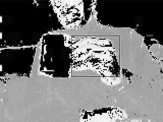
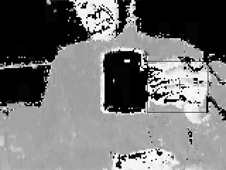
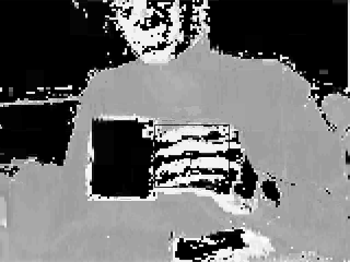
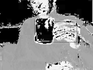
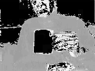
Figure 2 - Probability distribution of skin. High intensity values represent high probability of skin. The search window and centroid are also superimposed on each frame. The frames are in sequence from top to bottom in each row. The frames displayed are 0, 19, 39, 59, 79.

D. Conclusion

Object tracking is a very useful tool. Object can be tracked many ways including by color or by other features.

Tracking objects by difference frames is not always robust enough to work in every situation. There must be a static background and constant illumination to get great results. With this method, object can be tracked in only situations with transient optical flow. If the pixel values don't change, no motion will be detected.

The CAMSHIFT is a more robust way to track an object based on its color or hue. It is based after the MEAN SHIFT algorithm. CAMSHIFT improves upon MEAN SHIFT by accounting for dynamic probability distributions. It scales the search window size for the next frame by a function of the zeroth moment. In this way, CAMSHIFT  is very robust for tracking objects.

There are many variables in CAMSHIFT. One must decide suitable thresholds and search window scaling factors. One must also take into account uncertainties in hue when there is little intensity to a color. Knowing your distributions well helps to enable one to pick scaling values that help track the correct object. 

In any case, CAMSHIFT works well in tracking flesh colored objects. These object can be occluded or move quickly and CAMSHIFT usually corrects itself.

E. Appendix 
 

Source Code

Movies

The hand tracking movies have the follow format parameters:

Fps: 15.0000
Compression: 'Indeo3'
Quality: 75
KeyFramePerSec: 2.1429

Automatically updated parameters:
TotalFrames: 99
Width: 320
Height: 240
Length: 0
ImageType: 'Truecolor'
CurrentState: 'Closed'

F. 기타
CAM Shift Original Paper : Intel Technical Paper
http://isa.umh.es/pfc/rmvision/opencvdocs/papers/camshift.pdf


Hough 등 기타 Computer Vision Project Source/Tutorial 아래의 링크 참조
http://www.gergltd.com/cse486/
 

by 쿠리다쿠리 2011. 6. 21. 11:37
정리하면
Mean Shift는 non-parametric clustering 알고리즘 또는 과정으로 K-means Clustering(Duda, Hart & Stork, 2001)에 비해 Shape of Distribution, 클러스터의 개수 등에 대한 사전 정보를 요구하지 않는점이 가장 큰 차이점 이다.

원문:
Mean shift represents a general non-parametric mode finding/clustering procedure. In contrast to the classic K-means clustering approach (Duda, Hart & Stork,
2001), there are no embedded assumptions on the shape of the distribution nor the
number of modes/clusters.
(http://www.cse.yorku.ca/~kosta/CompVis_Notes/mean_shift.pdf 참조)

K-means Clustering Tutorial은 아래의 링크 참조
( http://www.autonlab.org/tutorials/kmeans11.pdf )

기타 기본 개념은 Andrew Moore의 Statistical Data Mining Tutorial 참조
(http://www.autonlab.org/tutorials/index.html)


by 쿠리다쿠리 2011. 6. 20. 22:25

From Wikipedia, the free encyclopedia

Empirical risk minimization (ERM) is a principle in statistical learning theory which defines a family of learning algorithms and is used to give theoretical bounds on the performance of learning algorithms.

Background

Consider the following situation, which is a general setting of many supervised learning problems. We have two spaces of objects X and Y and would like to learn a function \! h: X \to Y (often called hypothesis) which outputs an object y \in Y, given x \in X. To do so, we have in our disposal a training set of a few examples \! (x_1, y_1), \ldots, (x_m, y_m) where x_i \in X is an input and y_i \in Y is the corresponding response that we wish to get from \! h(x_i).

To put it more formally, we assume that there is a joint probability distribution P(x,y) over X and Y, and that the training set consists of m instances \! (x_1, y_1), \ldots, (x_m, y_m) drawn i.i.d. from P(x,y). Note that the assumption of a joint probability distribution allows us to model uncertainty in predictions (e.g. from noise in data) because y is not a deterministic function of x, but rather a random variable with conditional distribution P(y | x) for a fixed x.

We also assume that we are given a non-negative real-valued loss function L(\hat{y}, y) which measures how different is the prediction \hat{y} of a hypothesis from the true outcome y. The risk associated with hypothesis h(x) is then defined as the expectation of the loss function:

R(h) = \mathbf{E}[L(h(x), y)] = \int L(h(x), y)\,dP(x, y).

A loss function commonly used in theory is the 0-1 loss function: L(\hat{y}, y) = I(\hat{y} \ne y), where I(...) is the indicator notation.

The ultimate goal of a learning algorithm is to find a hypothesis \! h^* among a fixed class of functions \mathcal{H} for which the risk R(h) is minimal:

h^* = \arg \min_{h \in \mathcal{H}} R(h).

Empirical risk minimization

In general, the risk R(h) cannot be computed because the distribution P(x,y) is unknown to the learning algorithm (this situation is referred to as agnostic learning). However, we can compute an approximation, called empirical risk, by averaging the loss function on the training set:

\! R_\mbox{emp}(h) = \frac{1}{m} \sum_{i=1}^m L(h(x_i), y_i).

Empirical risk minimization principle states that the learning algorithm should choose a hypothesis \hat{h} which minimizes the empirical risk:

\hat{h} = \arg \min_{h \in \mathcal{H}} R_{\mbox{emp}}(h).

Thus the learning algorithm defined by ERM principle consists in solving the above optimization problem.

[edit] Properties


by 쿠리다쿠리 2010. 12. 9. 19:52
| 1 2 3 |