From Wikipedia:
이미지 Gradient를 계산하기 위한 방법은 Sobel, Canny등과 같은 다양한 Edge Filter를 이용하는 방법도 있을 수 있으나,
가장 간단한 방법은 다음과 같이 주변 Pixel간의 차이값을 이용하는 방법이다.

위의 수식을 입력 이미지에 대한 Filter mask(Matrix)형태로 표시하면 다음과 같다.

From Wikipedia atan2(x)
삼각법에서 atan2는 아크탄젠트함수에 대한 2 argument를 가지는 변형함수로 positive x축에서 좌표 (x, y)까지의 각도를 라디안(radian)으로 반환한다.
 atan2함수는 컴퓨터 프로그래밍 언어에서 처음 도입되었으나 현재는 과학, 엔지니어링 분야에서 일반적으로 사용되고 있다.
atan2(x, y)함수는 다음과 같은 조건으로 atan함수로 표현될 수 있다.

Notes:

• This produces results in the range (-π,π], which can be mapped to [0,2π) by adding 2π to negative values.

• Traditionally, atan2(0,0) is undefined.
  • The C function, and most other computer implementations, are designed to reduce the effort of transforming cartesian to polar coordinates and so always define atan2(0,0). On implementations without signed zero, or when given positive zero arguments, it is normally defined as 0. It will always return a value in the range [-π,π] rather than raising an error or returning a NaN (Not a Number).
  • Systems supporting symbolic mathematics normally return an undefined value for atan2(0,0) or otherwise signal that an abnormal condition has arisen.

• For systems, for example IEEE floating point, implementing signed zero, infinities, or Not a Number it is usual to implement reasonable extensions which may extend the range of values produced to include -π and -0. These also may return NaN or raise an exception when given a NaN argument.

아래는 아크탄젠트를 계산하기 위한 다양한 방법을 기술하고 있다.
아크탄젠트 연산은(삼각함수의 역함수 포함) 양변의 길이를 이용하여 각도값을 알고자 하는 경우에 사용한다.
아크 탄젠트는 라디안을 반환하므로 각도는 다음의 식으로 부터 구해질 수 있다
deg=atan(x)*180/pi()의 수식으로 구해진다
하드웨어상에서 이를 연산하기 윗한 수치해석적인 Arctangent의 연산 방법은 여러가지가 있으나 아래 문서(http://www.convict.lu/Jeunes/Math/arctan.htm)에 따르면 Look-up Table방식과 Polynomial 연산에 기반한 경우가 가장 정밀도가 높다고 한다.

Arctan(x) using CORDIC

1. The problem and some solutions

Sometimes, especially when navigating a robot, you'll have to determine a certain angle from the tangens-value. This is challenging because the RCX only works with small integer variables within the limits of -32768 and 32767. The arctan-function has to cover the range of 0...45 degrees e.a values of x between 0 and 1, first to avoid overflow errors or a division by zero problem at angles around 90 degrees. If the arctan has to be found for an angle alpha between 45 and 90 degrees (e.a. values of x above 1), you'll search for the arctan(1/x) and extract alpha=90-arctan(1/x).

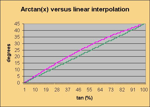
There are several possibilities to do the job, such as a look-up table, a linear or polynomial approximation or even a CORDIC algorithm. As you can see in the picture above, linear approximation will produce some big errors (~5°). Cumulated with other error sources, this will probably spoil your result.

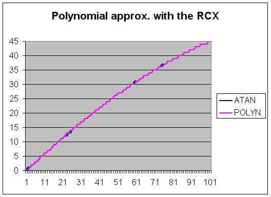
An acceptable result is given by polynomial approximation. The least squares technique gives the formula:

y = -0.30097 + 0.61955*x - 0.001659*x*x

x :number from 0..100%

y : angle from 0..45° as approximation of the atan function.

This formula has to be simplified for the RCX-use to always stay in the small-integer limits:

y ={ [-150 + 310 * x - (x*x DIV 2) - (x*x DIV 3) ] DIV 50 + 5 } DIV 10

This polynomial approximation gathers all the advantages: high speed (0.1 seconds), low memory, good accuracy!

We also tried a tricky approximation of This subroutine has been incorporated in both the second compass-sensor design and the pathfinder.

Here  the integral algorithm programmed first in PASCAL, then in RCX-Code.

 
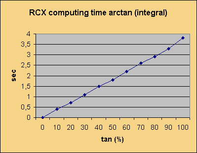
This is quite an interesting program-design. It does not affect much memory and has a precision of 1°, which is sufficient with the PEWATRON-sensor. But how about speed? In fact there are two major inconveniences that appear: first, the computing time is proportional to the input-value x, second, the RCX beeing a rather slow computer, it needs 3,6 seconds to calculate the arctan(1), which is quite a lot. In the case of the PEWATRON compass-programming this doesn't matter, because the sensor's recover-time stays around 2 seconds after turning, but in the case of the pathfinder this makes the robot react with an unstable delay. The actual course is never the real instant course but the course of some tenth of a second or even more in the past.

This delay-problem can be surrounded by a look-up table, where only few instructions have to be done.

Here an example of a look-up table. This program is not elegant, but it is very quick: 45° need only 0.2 seconds.
 

Download the RCX-Code

2. The CORDIC solution

CORDIC (COordinate Rotation DIgital Computer) is an iterative algorithm for calculating trigonometric functions and has been developed by J.E. Volder in 1959 (see "CORDIC Trigonometric Computing Technique", IRE Transactions on Electronic Computers, EC-8, Sept. 1959). It calculates the trig and even hyperbolic functions to any desired precision. The central idea is to rotate the phase of a complex number by a succession of constant values. Yes you should have paid attention in maths!
 

Given a complex value Z with the real component a, the imaginary component b, the phase phi:

Given a second complex value W = c + dj

Z ^. W = (a^.c - b^.d) + (a^.d + b^.c) j

Remember that when you multiply a pair of complex numbers, their phases are added and their magnitudes multiply. Similary, when you multiply a complex number by the conjugate of the other, the phase of the conjugated one is substracted, but the magnitudes still multiply. The conjugate of Z, Z* = a - bj.
 

For better comprehension have a look at the table below. You'll see that every rotation causes the magnitude to grow. The factor is dependent on L. If successive rotations are completed with L increasing progressively, the relative gain to the initial magnitude (called the CORDIC gain) grows, but tends to a limit value of 1.6467...
 

Exercise 1

We know the complex number Z = a + bj, for example Z₀ = 2 + 7j. Determine the phase phi.

CORDIC Solution:

This exercise is equivalent to fixing the arctan(2/7).

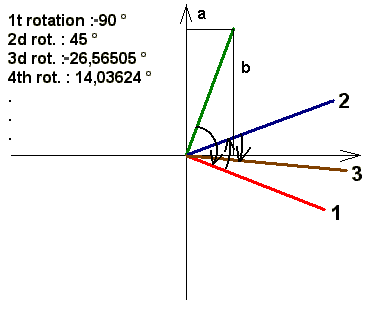
1. The CORDIC algorithm first lets you rotate by +90° if the imaginary argument b<0 and by -90° if the b>0. Example: Z₁ = 7 - 2j

2. Then rotate successively by atan(k), where k=+/-2^-L, L=0, 1, 2, 3, 4,.... . The decision of sign is always taken on the sign of the imaginary argument b. Obviously phi_i will tend towards 0. And this is the trick: we only have to add the well known values (which we poll from a look-up table) of the atan(k_i). At every computation these numbers will have the same absolute values. What only will change from case to case is the actual sign of k_i. If the actual phase of the rotated vector has sensibly reached 0, the opposite of sum=+/-90+S(atan(k_i)) gives us the phase of the initial complex number! ATTENTION: for this whole operation the real argument a must always be positive, e. a. angle values from -90 to +90°!!!

For better understanding have a look at the table below, or better try to calculate it by your own:
 

Download the Excel sheet

3. This computation gives us also the magnitude through the formula:

m(Z) = a_u / C_gain(u), where u is the index of the last operation with phi_u=0(+/-tolerance), b_u= 0 and a_u = m(Z_u)

This formula may be reduced to:

m(Z) = a_u / 1.6467, as shown above.

An RCX-program for this algorithm looks like:
 
 

 
Using this solution, we have a rather disappointing result: duration of a computation: 2.2 seconds; accuracy: 1-2°; high memory use. But we have learned some exciting program-technique!

Download the RCX-Code.

Exercise 2 : Calculate the square-root of a number x using CORDIC.

CONCLUSION

The best solution are the look-up table and the polynomial approximation.

In this article, I’ll show you how to rotate an image about its centre. 3 assignment methods will be shown,

• assign source pixels to destination pixels
• assign destination pixels from source pixels
• assign destination pixels from source pixels with bilinear interpolation

I’ll show you the code, then the results for comparison. So what’s bilinear interpolation?

Bilinear interpolation

Read up on linear interpolation first if you haven’t done so. “Bilinear” means there are 2 directions to interpolate. Let me illustrate.

In our case, we’re interpolating between 4 pixels. Visualise each pixel as a single point. Linearly interpolate between the top 2 pixels. Linearly interpolate between the bottom 2 pixels. Then linearly interpolate between the calculated results of the previous two.

You can expand on this concept to get trilinear interpolation.

LERPs is a short form of linear interpolations. When would trilinear interpolation be useful? Voxels, which is out of scope in this article.

Defining the centre of an image

I’m going to be fuzzy about this. I’m going to just take one pixel in the image and define it as the centre. This pixel is defined as having a horizontal index equal to half of its width (rounded down), and a vertical index equal to half its height (rounded down).

This means the image isn’t rotated about its “true” centre, but with a relatively large size, it won’t matter anyway. It’s not like you’re rotating an image of 5 pixel width and 3 pixel height, right?

The preparation part

The actual code is quite long, so I’m separating it into 4 parts.

• Initialisation and variable declaration
• Assigning source pixels to destination pixels
• Assigning destination pixels from source pixels
• Assigning destination pixels from source pixels with bilinear interpolation

It’s hard-coded with -30 degrees as the angle of rotation, but you can easily write it into a function.

// 30 deg = PI/6 rad
// rotating clockwise, so it's negative relative to Cartesian quadrants
const double cnAngle = -0.52359877559829887307710723054658;
// use whatever image you fancy
Bitmap bm = new Bitmap("rotationsource.jpg");
// general iterators
int i, j;
// calculated indices in Cartesian coordinates
int x, y;
double fDistance, fPolarAngle;
// for use in neighbouring indices in Cartesian coordinates
int iFloorX, iCeilingX, iFloorY, iCeilingY;
// calculated indices in Cartesian coordinates with trailing decimals
double fTrueX, fTrueY;
// for interpolation
double fDeltaX, fDeltaY;
// pixel colours
Color clrTopLeft, clrTopRight, clrBottomLeft, clrBottomRight;
// interpolated "top" pixels
double fTopRed, fTopGreen, fTopBlue;
// interpolated "bottom" pixels
double fBottomRed, fBottomGreen, fBottomBlue;
// final interpolated colour components
int iRed, iGreen, iBlue;
int iCentreX, iCentreY;
int iWidth, iHeight;
iWidth = bm.Width;
iHeight = bm.Height;

iCentreX = iWidth / 2;
iCentreY = iHeight / 2;

Bitmap bmSourceToDestination = new Bitmap(iWidth, iHeight);
Bitmap bmDestinationFromSource = new Bitmap(iWidth, iHeight);
Bitmap bmBilinearInterpolation = new Bitmap(iWidth, iHeight);

for (i = 0; i < iHeight; ++i)
{
    for (j = 0; j < iWidth; ++j)
    {
        // initialise when "throwing" values
        bmSourceToDestination.SetPixel(j, i, Color.Black);
        // since we're looping, we might as well do for the others
        bmDestinationFromSource.SetPixel(j, i, Color.Black);
        bmBilinearInterpolation.SetPixel(j, i, Color.Black);
    }
}

Some of it might not mean anything to you yet. Just wait for the rest of the code. You might want to read up on converting between raster, Cartesian and polar coordinates first before moving on.

Throwing values from source to destination

// assigning pixels from source image to destination image
for (i = 0; i < iHeight; ++i)
{
    for (j = 0; j < iWidth; ++j)
    {
        // convert raster to Cartesian
        x = j - iCentreX;
        y = iCentreY - i;

        // convert Cartesian to polar
        fDistance = Math.Sqrt(x * x + y * y);
        fPolarAngle = 0.0;
        if (x == 0)
        {
            if (y == 0)
            {
                // centre of image, no rotation needed
                bmSourceToDestination.SetPixel(j, i, bm.GetPixel(j, i));
                continue;
            }
            else if (y < 0)
            {
                fPolarAngle = 1.5 * Math.PI;
            }
            else
            {
                fPolarAngle = 0.5 * Math.PI;
            }
        }
        else
        {
            fPolarAngle = Math.Atan2((double)y, (double)x);
        }

        // the crucial rotation part
        fPolarAngle += cnAngle;

        // convert polar to Cartesian
        x = (int)(Math.Round(fDistance * Math.Cos(fPolarAngle)));
        y = (int)(Math.Round(fDistance * Math.Sin(fPolarAngle)));

        // convert Cartesian to raster
        x = x + iCentreX;
        y = iCentreY - y;

        // check bounds
        if (x < 0 || x >= iWidth || y < 0 || y >= iHeight) continue;

        bmSourceToDestination.SetPixel(x, y, bm.GetPixel(j, i));
    }
}
bmSourceToDestination.Save("rotationsrctodest.jpg", System.Drawing.Imaging.ImageFormat.Jpeg);

It should be fairly easy to read. Note the part about checking for the central pixel of the image. No rotation calculation necessary, so we assign and move to the next pixel. Note also the part about checking boundaries.

Finding values from the source

// assigning pixels of destination image from source image
for (i = 0; i < iHeight; ++i)
{
    for (j = 0; j < iWidth; ++j)
    {
        // convert raster to Cartesian
        x = j - iCentreX;
        y = iCentreY - i;

        // convert Cartesian to polar
        fDistance = Math.Sqrt(x * x + y * y);
        fPolarAngle = 0.0;
        if (x == 0)
        {
            if (y == 0)
            {
                // centre of image, no rotation needed
                bmDestinationFromSource.SetPixel(j, i, bm.GetPixel(j, i));
                continue;
            }
            else if (y < 0)
            {
                fPolarAngle = 1.5 * Math.PI;
            }
            else
            {
                fPolarAngle = 0.5 * Math.PI;
            }
        }
        else
        {
            fPolarAngle = Math.Atan2((double)y, (double)x);
        }

        // the crucial rotation part
        // "reverse" rotate, so minus instead of plus
        fPolarAngle -= cnAngle;

        // convert polar to Cartesian
        x = (int)(Math.Round(fDistance * Math.Cos(fPolarAngle)));
        y = (int)(Math.Round(fDistance * Math.Sin(fPolarAngle)));

        // convert Cartesian to raster
        x = x + iCentreX;
        y = iCentreY - y;

        // check bounds
        if (x < 0 || x >= iWidth || y < 0 || y >= iHeight) continue;

        bmDestinationFromSource.SetPixel(j, i, bm.GetPixel(x, y));
    }
}
bmDestinationFromSource.Save("rotationdestfromsrc.jpg", System.Drawing.Imaging.ImageFormat.Jpeg);

The key difference here is the use of the rotation angle. Instead of adding it, we subtract it. The reason is, we rotate source pixels 30 degrees clockwise and assign it to destination pixels. But from destination pixels, we get source pixels which are rotated 30 degrees anticlockwise. Either way, we get a destination image that's the source image rotated 30 degrees clockwise.

Also compare the assignment, noting the indices:

bmSourceToDestination.SetPixel(x, y, bm.GetPixel(j, i));
bmDestinationFromSource.SetPixel(j, i, bm.GetPixel(x, y));

x and y variables are calculated and thus "messy". I prefer my messy indices on the right. There's a practical reason for it too, which will be evident when I show you the rotation results.

Image rotation code with bilinear interpolation

// assigning pixels of destination image from source image
// with bilinear interpolation
for (i = 0; i < iHeight; ++i)
{
    for (j = 0; j < iWidth; ++j)
    {
        // convert raster to Cartesian
        x = j - iCentreX;
        y = iCentreY - i;

        // convert Cartesian to polar
        fDistance = Math.Sqrt(x * x + y * y);
        fPolarAngle = 0.0;
        if (x == 0)
        {
            if (y == 0)
            {
                // centre of image, no rotation needed
                bmBilinearInterpolation.SetPixel(j, i, bm.GetPixel(j, i));
                continue;
            }
            else if (y < 0)
            {
                fPolarAngle = 1.5 * Math.PI;
            }
            else
            {
                fPolarAngle = 0.5 * Math.PI;
            }
        }
        else
        {
            fPolarAngle = Math.Atan2((double)y, (double)x);
        }

        // the crucial rotation part
        // "reverse" rotate, so minus instead of plus
        fPolarAngle -= cnAngle;

        // convert polar to Cartesian
        fTrueX = fDistance * Math.Cos(fPolarAngle);
        fTrueY = fDistance * Math.Sin(fPolarAngle);

        // convert Cartesian to raster
        fTrueX = fTrueX + (double)iCentreX;
        fTrueY = (double)iCentreY - fTrueY;

        iFloorX = (int)(Math.Floor(fTrueX));
        iFloorY = (int)(Math.Floor(fTrueY));
        iCeilingX = (int)(Math.Ceiling(fTrueX));
        iCeilingY = (int)(Math.Ceiling(fTrueY));

        // check bounds
        if (iFloorX < 0 || iCeilingX < 0 || iFloorX >= iWidth || iCeilingX >= iWidth || iFloorY < 0 || iCeilingY < 0 || iFloorY >= iHeight || iCeilingY >= iHeight) continue;

        fDeltaX = fTrueX - (double)iFloorX;
        fDeltaY = fTrueY - (double)iFloorY;

        clrTopLeft = bm.GetPixel(iFloorX, iFloorY);
        clrTopRight = bm.GetPixel(iCeilingX, iFloorY);
        clrBottomLeft = bm.GetPixel(iFloorX, iCeilingY);
        clrBottomRight = bm.GetPixel(iCeilingX, iCeilingY);

        // linearly interpolate horizontally between top neighbours
        fTopRed = (1 - fDeltaX) * clrTopLeft.R + fDeltaX * clrTopRight.R;
        fTopGreen = (1 - fDeltaX) * clrTopLeft.G + fDeltaX * clrTopRight.G;
        fTopBlue = (1 - fDeltaX) * clrTopLeft.B + fDeltaX * clrTopRight.B;

        // linearly interpolate horizontally between bottom neighbours
        fBottomRed = (1 - fDeltaX) * clrBottomLeft.R + fDeltaX * clrBottomRight.R;
        fBottomGreen = (1 - fDeltaX) * clrBottomLeft.G + fDeltaX * clrBottomRight.G;
        fBottomBlue = (1 - fDeltaX) * clrBottomLeft.B + fDeltaX * clrBottomRight.B;

        // linearly interpolate vertically between top and bottom interpolated results
        iRed = (int)(Math.Round((1 - fDeltaY) * fTopRed + fDeltaY * fBottomRed));
        iGreen = (int)(Math.Round((1 - fDeltaY) * fTopGreen + fDeltaY * fBottomGreen));
        iBlue = (int)(Math.Round((1 - fDeltaY) * fTopBlue + fDeltaY * fBottomBlue));

        // make sure colour values are valid
        if (iRed < 0) iRed = 0;
        if (iRed > 255) iRed = 255;
        if (iGreen < 0) iGreen = 0;
        if (iGreen > 255) iGreen = 255;
        if (iBlue < 0) iBlue = 0;
        if (iBlue > 255) iBlue = 255;

        bmBilinearInterpolation.SetPixel(j, i, Color.FromArgb(iRed, iGreen, iBlue));
    }
}
bmBilinearInterpolation.Save("rotationbilinearinterpolation.jpg", System.Drawing.Imaging.ImageFormat.Jpeg);

This part is similar to the destination-from-source part, with a lot more calculations. We have to find the 4 pixels that surrounds our "true" position-calculated pixel. Then we perform linear interpolation on the 4 neighbouring pixels.

We need to interpolate for the red, green and blue components individually. Refer to my article on colour theory for a refresher.

Pictures, pictures!

After doing all that, we're finally done. Let me show you my source image first.

I added the marble cylinder for emphasising image quality. I needed something that's straight (vertically or horizontally) in the source image.

Here's what we get after rotating with the source-to-destination method:

Note the speckled black pixels dotted all over. This is because some of the destination pixels (which are within the image bounds) were unassigned.

Note also that the specks even form patterns. This is due to the sine and cosine functions, and the regularity of pixel width and height. Sine and cosine are periodic functions. Since pixel indices are regular, therefore sine and cosine results are regular too. Hence, calculations regularly fail to assign pixel values.

There might be source pixels that have the same calculated destination pixel (due to sine and cosine and rounding). This also implies that there might be anti-gravity destination pixels that no source pixel can ever matched to! I haven't verified this, but it seems a possibility.

Still think you should iterate over the source (image/array) instead of over the destination?

Next, we have the image result of the destination-from-source method:

Compare the quality with the source-to-destination part. No missing pixels. It's still sort of grainy though. This is because some of the destination pixels get their values from the same source pixel, so there might be 2 side-by-side destination pixels with the same colour. This gives mini blocks of identical colour in the result, which on the whole, gives an unpolished look.

Now, we have the bilinear interpolation incorporated version.

It looks smoother, right? Note the straight edge of the marble cylinder. Compare with the image result without bilinear interpolation.

I might do a version with cubic interpolation for even smoother results, but I feel the bilinear version is good enough for now. Have fun!

Interpolation is a method of calculating a value from a set of given values. We’ll be looking at interpolation with a bias towards image processing, but the theory can be generalised for other purposes. You’ve probably already solved some interpolation problems without knowing it. Let me give you an example.

A distance problem

Suppose there are 3 towns A, B, C and they happen to lie on a straight line, in that order. B is 5 kilometres away from A, and C is 15 kilometres away from A. If you travel one quarter of the way from town B to town C, how far are you from town A?

To solve it, you can figure out the distance between B and C, which is 15 – 5 = 10 km. One quarter of the way means 1/4 * 10 = 2.5 km. Then add the distance between A and B to this and you have 5 + 2.5 = 7.5 km.

Linear interpolation

If you visualise the problem as interpolating between 2 points, then B becomes the point p0 with a value of 5 (km) and C becomes the point p1 with a value of 15 (km). The usual variable used is t, so the generic formula is:
f(t) = (1 – t) * p0 + t * p1, where t lies between 0 and 1 inclusive.

Using this, we have
f(1/4) = (1 – 1/4) * 5 + 1/4 * 15
= 3/4 * 5 + 1/4 * 15
= 7.5

This is linear interpolation. Linearity refers to the power of the variable t, which is 1. Note that there’s no stopping you from using negative values of t or values greater than 1.

Suppose you travelled from B to A one quarter of the distance between B and C. How far are you from town A?
f(-1/4) = (1 – (-1/4)) * 5 + (-1/4) * 15
= 5/4 * 5 – 1/4 * 15
= 2.5

Suppose you travelled from B to C and went past C by a quarter of the way. How far are you from town A?
f(5/4) = (1 – 5/4) * 5 + 5/4 * 15
= -1/4 * 5 + 5/4 * 15
= 17.5

What happens if you get a negative result?
f(-1) = (1 – (-1)) * 5 + (-1) * 15
= 2 * 5 – 15
= -5

It means you’re 5 kilometres away from town A. You’re just in the opposite direction from towns B and C. The calculation result is correct. It’s how you interpret the value.

Applications in image processing

A common operation in image processing is manipulating height maps. Height maps are usually greyscale bitmap files where a white pixel (RGB values are 255 for all 3) is the highest point, and a black pixel (RGB values are 0 for all 3) is the lowest point.

You know enlarging photographs can give you some weird results. What happens is you’re trying to fill in the blanks in a larger image using values from the original image. Where do you think the image editing software comes up with values? Interpolation.

If you think of the red, green and blue values of image pixels as 3 different “height maps”, then you’re just performing interpolation on 3 values. Suppose we’re talking about linear interpolation between two pixels. You’ll interpolate between the red component of the 2 pixels and get a value. Similarly you do it for the green and blue components. The calculated results of the red, green and blue become the interpolated colour.

Cubic Bezier interpolation

There are all kinds of cubic curves available. The Catmull–Rom spline, the non-uniform rational B-spline (NURBS) and I didn’t really want to write anything on the subject after I remember my Hermite splines… I love Bezier curves though, so I thought maybe I can write something with that.

Instead of 2 points used in linear interpolation, cubic interpolation uses 4 points. To illustrate, suppose you’re on an undulating plain with small hills undulating in their usual carefree manner. You’re in between two such (undulating) hills and you want to find out how high you are.

Instead of linear interpolating your way through these two (undulating) hills, the better way will be to interpolate with another 2 (undulating) hills! Ok, I’m stopping with the undulating thing…

The Bezier curve equation looks like this:
B(t) = (1-t)^3 * p0 + 3*(1-t)^2 * t * p1 + 3*(1-t)* t^2 * p2 + t^3 * p3
where p0, p1, p2, p3 are the (height) values, and t lies between 0 and 1 inclusive.

You will be between p1 and p2. Let’s also assume that the hills are equidistant from each other. Like the pixels on an image, the hills shall be of equal distance from its neighbour.

Because of this equidistant property, p1 is 0.33 (roughly 1/3) units away from p0, p2 is 0.67 (roughly 2/3) units away from p0 and p3 is 1 unit away from p0.

How do you know what’s the value of t to use? You might be able to calculate the t if you do linear interpolation between p1 and p2. But that t value is different from the t value in the Bezier curve.

Ahhh… once you get the t-linear value, you interpolate with 0.33 and 0.67 to get the t-Bezier value. Confused? Suppose you’re one quarter way from p1 to p2. Your t-linear value is 1/4. Interpolate that with 0.33 and 0.67 to get
f(1/4) = (1 – 1/4) * 0.33 + 1/4 * 0.67
= 0.415

And 0.415 is your t-Bezier value. Voila!

You skipped the quadratic power!

I know. It’s logical to think that there’s a power 2 somewhere. But there isn’t. There is one fundamental flaw with quadratic interpolation. Which segment do you use?

In closing

Interpolation is just a method of creating data values using a set of existing data. What those created values mean is up to you to interpret.

In image processing, interpolation can be used to fill in blanks when enlarging an image. It doesn’t guarantee that the enlarged image looks good. Image processing is very much an aesthetic-based operation. I’ll talk a bit more on this when I get to writing code to rotate images.