CAMSHIFT Algorithm
The CAMSHIFT algorithm is based on the MEAN SHIFT algorithm. The MEAN SHIFT algorithm works well on static probability distributions but not on dynamic ones as in a movie. CAMSHIFT is based principles of the MEAN SHIFT but also a facet to account for these dynamically changing distributions.
CAMSHIFT's is able to handle dynamic distributions by readjusting the search window size for the next frame based on the zeroth moment of the current frames distribution. This allows the algorithm to anticipate object movement to quickly track the object in the next scene. Even during quick movements of an object, CAMSHIFT is still able to correctly track.
The CAMSHIFT algorithm is a variation of the MEAN SHIFT algorithm.
CAMSHIFT works by tracking the hue of an object, in this case, flesh color. The movie frames were all converted to HSV space before individual analysis.
CAMSHIFT was implemented as such:
1. Initial location of the 2D search window was computed.
2. The color probability distribution is calculated for a region slightly bigger than the mean shift search window.
3. Mean shift is performed on the area until suitable convergence. The zeroth moment and centroid coordinates are computed and stored.
4. The search window for the next frame is centered around the centroid and the size is scaled by a function of the zeroth movement.
5. Go to step 2.
The initial search window was determined by inspection. Adobe Photoshop was used to determine its location and size. The inital window size was just big enough to fit most of the hand inside of it. A window size too big may fool the tracker into tracking another flesh colored object. A window too small will mostly quickly expand to an object of constant hue, however, for quick motion, the tracker may lock on the another object or the background. For this reason, a hue threshold should be utilized to help ensure the object is properly tracked, and in the event that an object with mean hue not of the correctly color is being tracked, some operation can be performed to correct the error.
For each frame, its hue information was extracted. We noted that the hue of human flesh has a high angle value. This simplified our tracking algorithm as the probability that a pixel belonged to the hand decreased as its hue angle did. Hue thresholding was also performed to help filter out the background make the flesh color more prominent in the distributions.
The zeroth moment, moment for x, and moment for y were all calculated. The centroid was then calculated from these values.
xc = M10 / M00; yc = M01 / M00
The search window was then shifted to center the centroid and the mean shift computed again. The convergence threshold used was T=1. This ensured that we got a good track on each of the frames. A 5 pixel expansion in each direction of the search window was done to help track movement.
Once the convergent values were computed for mean and centroid, we computed the new window size. The window size was based on the area of the probability distribution. The scaling factor used was calculated by:
s = 1.1 * sqrt(M00)
The 1.1 factor was chosen after experimentation. A desirable factor is one that does not blow up the window size too quickly, or shrink it too quickly. Since the distribution is 2D, we use the sqrt of M00 to get the proper length in a 1D direction.
The new window size was computed with this scaling factor. It was noted that the width of the hand object was 1.2 times greater than the height. This was noted and the new window size was computed as such:
W = [ (s) (1.2*s) ]
The window is centered around the centroid and the computation of the next frame is started
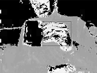
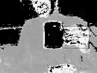
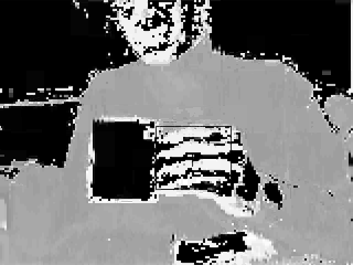
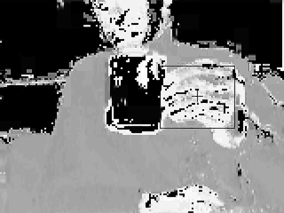

Figure 2 - Probability distribution of skin. High intensity values represent high probability of skin. The search window and centroid are also superimposed on each frame. The frames are in sequence from top to bottom in each row. The frames displayed are 0, 19, 39, 59, 79.
D. Conclusion
Object tracking is a very useful tool. Object can be tracked many ways including by color or by other features.
Tracking objects by difference frames is not always robust enough to work in every situation. There must be a static background and constant illumination to get great results. With this method, object can be tracked in only situations with transient optical flow. If the pixel values don't change, no motion will be detected.
The CAMSHIFT is a more robust way to track an object based on its color or hue. It is based after the MEAN SHIFT algorithm. CAMSHIFT improves upon MEAN SHIFT by accounting for dynamic probability distributions. It scales the search window size for the next frame by a function of the zeroth moment. In this way, CAMSHIFT is very robust for tracking objects.
There are many variables in CAMSHIFT. One must decide suitable thresholds and search window scaling factors. One must also take into account uncertainties in hue when there is little intensity to a color. Knowing your distributions well helps to enable one to pick scaling values that help track the correct object.
In any case, CAMSHIFT works well in tracking flesh colored objects. These object can be occluded or move quickly and CAMSHIFT usually corrects itself.
E. Appendix Source Code
Movies
The hand tracking movies have the follow format parameters:
Fps: 15.0000

Compression: 'Indeo3'

Quality: 75

KeyFramePerSec: 2.1429


Automatically updated parameters:

TotalFrames: 99

Width: 320

Height: 240

Length: 0

ImageType: 'Truecolor'

CurrentState: 'Closed'


F. 기타

CAM Shift Original Paper : Intel Technical Paper

http://isa.umh.es/pfc/rmvision/opencvdocs/papers/camshift.pdf


Hough 등 기타 Computer Vision Project Source/Tutorial 아래의 링크 참조

http://www.gergltd.com/cse486/
 또는
또는  로 주어진다.


 (often called hypothesis) which outputs an object
  , given
  . To do so, we have in our disposal a training set of a few examples
  where
where  is an input and
  is the corresponding response that we wish to get from
  .
. which measures how different is the prediction
  of a hypothesis from the true outcome
 ![R(h) = \mathbf{E}[L(h(x), y)] = \int L(h(x), y)\,dP(x, y).](http://upload.wikimedia.org/math/f/c/5/fc5a0829e5d2623238d89a47fcf2a701.png)
 , where
  among a fixed class of functions
  for which the risk

 which minimizes the empirical risk:


RECENT COMMENT